Congruency-Based
Hysteresis Model
for
Transient Simulation
The present website contains a Demo version of a static hysteresis model that is an extension of the history-dependent hysteresis model described in [14]. The necessity for such an extension is described in Introduction.
This site is also supplied by a Demo version of the Classical Preisach model (CPM) with a Lorentzian PDF.
The authors of this Demo (S.E.Zirka and Y.I.Moroz) are with the Dnepropetrovsk National University, Ukraine
49050, Dnepropetrovsk, Naukova str. 13, Ukraine, e-mail: zirka@email.dp.ua
I. Introduction
The
reliability of modeling and the quality of design of any device containing a
magnetic core is greatly influenced by the adequacy of the hysteresis model
employed and, in particular, by its ability to reproduce the magnetization
history. This is especially true with
respect to modern electrical machines and other equipment whose laminated cores
are magnetized by nonsinusoidal voltage [1], [2]. Such an excitation causes
complex shapes of the magnetization curves and their qualitative differences in
different “layers” of the conducting ferromagnetic sheet (at the nodes of a
finite-difference grid or finite elements corresponding to separate
layers). It
is important to note that the dynamic magnetization of such layers is described
by employing static B(H)
curves. In the case where excess losses
should be taken into account, this can be done by introducing a time lag of the
induction B behind the applied field H [2]. This transforms the static hysteresis model into a dynamic one
and, remarkably, the static (basic) component of the
dynamic hysteresis model obtained may be of any type
and nature (history-dependent or history-independent, Preisach or
non-Preisach). Thus, it is of
fundamental importance to develop a quasi-static procedure, which allows one to
predict the behavior of a ferromagnetic material (its induction В or magnetization М) corresponding to an arbitrary change in the field Н.
It is well known that this behavior is determined by the prehistory of
the process, where every sheet layer (the node of the grid) has its own
history. These nodal histories must be
traced and updated when solving the boundary value problem (BVP) describing the magnetization transient. Because of its multiple recalls, such a
procedure should be as simple as possible but
also sufficiently accurate.
In the present website we present a history-dependent hysteresis model (HDHM)
based on direct use of experimental
first-order reversal curves only (the major loop branches belong to their
family). This means that any
first-order reversal curve is reproduced exactly
by such a model, and the prediction algorithm is engaged starting from the
construction of second-order reversal curves.
Despite the multiplicity of hysteresis models developed to date, there
is no adequate model possessing these qualities. The HDHM with the same input data most often used for studying
the transient and steady-state regimes is the classical Preisach model (CPM) [3]. Its intrinsic properties are the return-point memory and
the specific H-congruency of the
produced curves (all branches starting from turning points with the same field H have the same shape, independent of history). It is well known that real materials do not
obey the H-congruency of the
CPM. The same is also true for the M-congruency of the model [4],
the skew congruency of the moving model [5] or the nonlinear congruency of the
product model [6]. As a result, even
the modeled major loop and first-order reversal
curves differ from experimental ones,
and some nonphysical behavior of the calculated curves can arise. The most unwanted feature is a negative slope of the reversal curve, (examples can be
found in [7, Fig. 6]), that leads to instability of the magnetodynamic
equations solved.
The
known iterative procedures aimed at the elimination of the nonphysical negative
values of the Preisach distribution function, PDF, (described in [8] for the
moving model, and in [9], [10] for the CPM), seem to be quite complex and lead
to the mentioned difference between calculated and experimental first-order
curves. It should be noticed that
first-order reversal curves are reproduced exactly by models [11], [12] which
are based on the concept of equal vertical chords [13]. However the
implementation of this concept requires the measurement of first- and
second-order reversal curves, and what is more important, it does not guarantee
that transition curves with negative slopes do not occur starting from the
third order reversal curves. This was
not noticed by the authors of the concept, but becomes evident in the course of
solving the BVP with complex magnetic trajectories.
The approach where negative slopes are impossible by definition is
the direct use of experimental magnetization
curves without their reconstruction. It is instructive, in this connection, to analyze the congruency based
technique proposed in [3, formulas (1.75), (1.76)]
and its modification suggested in [12, formulas (4), (5)]. Because exclusively experimental first-order curves are used in such techniques, they can be referred to as CPM-E. As such the CPM-E approach used in [3]
and [12] is an uncritical extension of the H-congruency that is valid for the CPM
to a real material which does not possess this property. As a result, the CPM-E [3] leads to a discontinuity
of the magnetic trajectories, whereas the CPM-E [12] gives unclosed minor
loops.
In the present model we renew the concept of the congruency
by constructing any second and higher order reversal curve, whose overall
dimensions (ODs) DH and
DB are always known
in the HDHM, by using internal segments
of the experimental first-order reversal curves with the required ODs.
The question of how to choose or approximate the specific segment arises since the number of
such segments (transplants) belonging to the experimental or interpolated
first-order curves is infinite. It
has been proposed in [14] to close a minor loop by using a transplant which
is the nearest to the formed loop in the B- (or M-) direction.
In fact, this was an attempt to perfect the B-congruency
observed by Madelung [15] who noticed a resemblance of the transition curves
starting from turning points with the same induction B. In the model proposed we expand the transplant
search region to the whole B-H (or
M-H) plane. This allows us to change the
shape of the reversal curve, and
consequently the area enclosed by the minor loop. Such an increase in the model degrees of freedom enables one to carry out a fine adjustment
of the model, taking into account, for example, the second order reversal
curves (if available), and varying, in such a way, the energy losses calculated
in the course of transient analysis. These
details will be described in a full-length paper written in coauthorship
with Prof. A. J. Moses and Dr. P. Marketos (Cardiff University, UK).
II. Magnetization
regularities reproduced by the model
Despite the wide variety of characteristics of different magnetic media, some general regularities are observed in their magnetization processes. These regularities have been described in the early twentieth century [15] and are known as Madelung’s rules (see e.g. [16]).
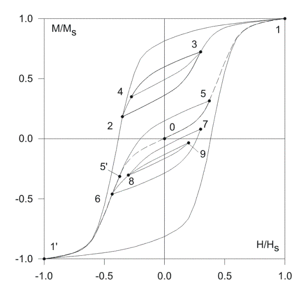
Considering the
hysteresis curves in Fig. 1 (constructed with the proposed HDHM), the
experimentally established magnetization rules [15] can be stated as follows.

Fig. 1. Transition curves illustrating Madelung’s rules (the major static loop is scanned from [17]).
1) The path of any first-order reversal curve is uniquely determined by the
coordinates of the reversal point, from which this curve emanates.
2) If any point 3 of curve 2-3-1 becomes a new
reversal point, then curve 3-4-2 originating at point 3 returns to the initial
point 2 (return-point memory).
3) If point 4 of curve 3-4-2 becomes the newest
reversal point and the transition curve 4-3 extends beyond the point 3, it will
pass along the section 3-1 of curve 2-3-1, as if the previous closed loop 3-4-3
did not exist at all (wiping-out property).
4) All transition curves which start from the
reversal points having the same ordinates and sign of induction (magnetization)
increment can be brought into coincidence by their parallel motion along the H-axis (B-congruency of the reversal curves).
5) If some point 5 of the initial magnetization curve becomes a reversal point, then the transition curve which starts from point 5 reaches point 5' which is symmetrical with respect to point 5 about the origin 0. At the same time, rules 2 and 3 remain in force here as everywhere (this is illustrated by the closed loops 6-7-6 and 8-9-8). (This rule has been formulated in [18] as a supplement to the regularities described by Madelung and can be useful when modeling a transient originating from the demagnetized state).
The proposed model reproduces rules 1, 2, 3 immediately. To reproduce
the rule 4, a demagnetizing ac procedure should be first carried out (it can
be performed by using the Demo proposed).
III. Input (Material) Data Required
The model is equally suited for both the B(H) and M(H)
dependencies. It is impossible for a model to be accurate without using first-order
reversal curves of a given material. Being
the unique characteristics of a ferromagnet, these curves should be obtained
by experiment. In the case when experimental
first-order curves are not available, they can be generated by means of the
procedure suggested in Appendix to [14] or even drawn by hand (this need only
be done once for a given material).
The model imposes no restrictions both on the shape of the major loop and on the number of first-order curves employed, although 10-15 curves are still desirable to provide an engineering accuracy.
On this website, we post the
following 5 sets of input data for both particulate recording media and soft
crystalline alloys.
1. Data file ‘Mayer-89.txt’ contains the experimental data of the g-Fe2O3material scanned from [17]. To avoid sharp turns in the broken experimental curves [17], we have smoothed these curves by inserting some extra points and interpolating them by cubic splines.
2. Data file ‘Dupre-98.txt’ contains the experimental data of non-oriented steel. The major loop of the material has been obtained by exploiting a standard Epstein frame. First-order reversal curves of the material have been constructed by using the procedure described in [14].
3. Data file ‘Dupre-99.txt’ contains the experimental data of another non-oriented steel. Both the major loop and first-order curves have been obtained with the Epstein frame.
4. Data file ‘Wolf-NO.txt’ contains the experimental data of non-oriented steel. Both the major loop and first-order curves have been obtained with an Epstein frame.
5. Data file ‘Wolf-GO.txt’ contains the experimental data of grain-oriented steel. Both the major loop and first-order curves have been obtained with the Epstein frame.
IV. How
to Install the Demo
1) Download the Demo.zip archive
from the site. It contains an executable file of the Demo code (‘Demo.exe’)
and five data (material) files (‘Mayer-89.txt’, ‘Dupre-98.txt’, ‘Dupre-99.txt’,
‘Wolf-NO.txt’, ‘Wolf-GO.txt’).
2) UnZip the Demo.zip with WinZip into a directory. No further installation is required.
3) If necessary, the Demo version of static (rate independent)
CPM can be also installed. With this purpose, download the Preisach-demo.zip
archive from the site. It contains an executable file of the Demo CPM code
(‘Preisach-demo.exe’)
V. How
to Use the Demo
(Short Manual of April 29, 2003)
This program works under Microsoft Windows (95 or higher) in the 16-bit
screen modes (for example 256 colors, High colors, but not True
colors).
0) Execute the ‘Demo.exe’.
1) To initiate modeling, select the menu item:
“File” ® “Open data file...”.
2) Choose a specific material data among the following data files:
2.1. ''Mayer-89.txt''.
2.2. ''Dupre-98.txt''.
2.3. ''Dupre-99.txt''.
2.4. ''Wolf-NO.txt''.
2.5. ''Wolf-GO.txt''.
3) Use the left
mouse button to set the H-coordinate of the next reversal (the mouse
pointer should be within the frame of the plot, in this case
current H- and B-coordinates are shown at the bottom of the
frame).
Use the right mouse button to construct the corresponding transition
curve.
4) To set the next reversal point numerically, you may also use:
Menu item “State” ® “Input Hn...”, press “Execute” when ready.
5) To save the trajectory obtained in a text file (this option is unavailable in the Demo version):
Menu item “File” ® “Save results…” ® Input a file name in the window.
6) Using this program, you may also simulate a demagnetizing AC procedure with up to 900 reversal points:
Menu item “State”® ”Input Hn...”, set 0 in the Hn input window, select item “Gradual spiral approach to Hn”, and set the number of cycles (<451), press “Execute” when ready.
Note: It may require about a minute to complete the procedure for a large number of reversals.
7) To study in more detail a fragment of the trajectory obtained, you
can change the scales of both the H- and B-axes:
Menu item “State”® ”Axes…”, set the values, press “OK”.
8) Default setting of the initial state is the negative saturation (–Hs). In the case when the initial state of the positive saturation (+Hs) is desirable, use immediately after opening a data file:
Menu item “State”® ”Settings…”, choose Ho=Hs, OK.
9) To initiate modeling with another material:
Menu item “File” ® ”Close workspace”, and initiate the simulation beginning from item 1 above.
The manual for the Preisach-demo.exe is the same as above with the exception of item 2, where the value of the conventional coercivity should be entered instead of the file name.
VI. Results
and Discussion
The use of the Demo
in modeling complex trajectories is illustrated by Fig. 2, where experimental [3], [17] and calculated curves are almost indistinguishable

Fig. 2. Comparison of the experimental transition curves from [3] (solid lines) with the curves predicted by the proposed model (dashed lines)
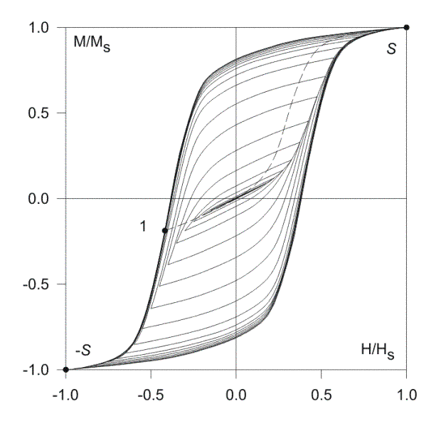
The possibilities of the history-dependent model are also illustrated
by an uninterrupted four-phase process shown in Fig. 3. Its first phase
(a demagnetizing AC procedure) emanates from the negative saturation and completes
at the origin. The second phase originates
from the demagnetized state and represents the continuous magnetization up
to the positive saturation (reversal point S). The trajectory showing
this phase, successively passes through all the turning points in the first
quadrant, and the closed minor loops obtained are wiped out from the model
memory in accordance with Madelung rule 3.
The third phase
of the process is a transition from point S to point 1 of the remanent
coercivity. The latter point is characterized by first-order reversal curve
1-S passing through the origin (this final phase of the process is
shown in Fig. 3 by dashed line). As seen from Fig. 3, first-order curve 1-S
traced during the forth phase of the process substantially differs from the
initial curve which is a locus of the minor loops extrema obtained in the
course of the demagnetizing procedure. It is clear that the initial curve
constructed with the HD model would depend on the preceding demagnetizing
procedure. However, the difference between the initial curves following the
demagnetization with large numbers of reversals (say 50 and 100) is negligible
small. This allows us to bring these reversals into the model memory (the
same history in each nodal memory) and use them in evaluating the transient
when a symmetric steady-state dynamic loop is required.

Fig. 3. Uninterrupted process constructed by means of the proposed model
If the field reversal occurs on the ascending
branch of the imaginary initial curve formed by the minor loop extrema in
the first quadrant, then corresponding reversal curve returns to the point
of the previous reversal which is situated on the ascending branch of the
imaginary initial curve and, by virtue of the minor loop symmetry, is symmetric
to the current reversal point about the origin. Consequently, rule 5 is performed
automatically after demagnetizing process with a large number of reversals
if the model satisfies rules 2 and 3. This is illustrated by Fig. 1 where
uninterrupted curve 0-5-5'-6-7-8-9-8-6-1' has been built after the demagnetizing
procedure like that shown in Fig. 3 but with 120 reversals instead of 20 ones.
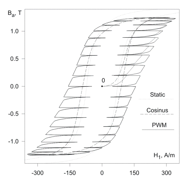
The model proposed can be incorporated
into a transient simulator [1, 2, 19, 20], where boundary value problem for
a conducting ferromagnetic lamination is solved. As
an example of the problem where both the transient and steady-state regimes
can not be evaluated without hysteresis modeling, we consider the dynamic
process in a single lamination subjected to the PWM voltage supply (the fundamental
frequency f=50 Hz, the carrier frequency fc=1 kHz, the modulation index m=0.45). Static hysteresis loop
of the magnetic material (non-oriented steel with the thickness d=0.51
mm and the conductivity s=2.63·106 S/m) is shown in Fig.
4 by dashed lines. Before applying the excitation, the demagnetizing ac procedure
consisting of 100 reversals has been simulated. The first three periods of
the start-up transient calculated by a finite-difference scheme [19] are shown
in Fig. 4 by solid line.

Fig. 4. Dynamic magnetization curves calculated for PWM and cosine
voltage excitations
In the present website we have restricted our attention to the model possessing
the wiping-out (deletion) property. The conventional definition of this property
results in calculated minor loops immediately stable after the first traversal.
In real media some number of traversals may be required to reach the static
loops, so accommodation properties of the media should be taken into account
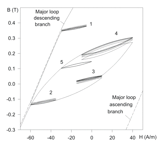
for such materials. A model including accommodation can be developed as an
extension of the nonaccommodating model described above. Our numerical experiments
in this direction are illustrated by an uninterrupted curve shown in Fig.
5.
Fig. 5. Uninterrupted process constructed with accommodating model
The process shown in Fig. 5 includes 5 separate cyclings of the field. It is interesting that during one of them (cycling 5 consists of 10 reversals) the accommodation does not show itself. A detail experimental investigation of the accommodation behavior of real media is needed to complete this model.
Acknowledgment
We are grateful to Dr. L.Dupre (Ghent University, Belgium) for providing
experimental data of the non-oriented steels (materials 2 and 3 above). Experimental data of the non-oriented and grain-oriented steels (materials
4 and 5 above) were obtained by the courtesy of Prof. A.J. Moses and Dr. P. Marketos (Cardiff University, UK).
REFERENCES
1. L.R.Dupre, R.Van Keer, J.A.A.Melkebeek, Y.I.Moroz and S.E.Zirka, “Hysteresis models for transient simulation,” Lect. Notes in Comp. Sci. and Eng., vol. 18, pp. 105-112, Springer-Verlag, Berlin, 2001.
2. S.E.Zirka, Y.I.Moroz, P.Marketos, A.J.Moses, “Modeling losses in electrical steel laminations,” IEE Proc.- Sci. Meas. Technol., vol. 149, no. 5, pp. 218-221, Sept. 2002.
3. I.D.Mayergoyz, Mathematical Models of Hysteresis. Springer-Verlag, New York, 1991.
4. V.Basso and G.Bertotti, “Hysteresis models for the description of domain wall motion”, IEEE Trans. Magn., vol. 32, no. 5, pp. 4210-4212, 1996.
5. E.Della Torre, “Effect of interaction on the magnetization of single domain particles,” IEEE Trans. Audio Electroacoust., vol. 14, no. 2, pp. 86-93, 1966.
6. G.Kadar, “On the Preisach function of ferromagnetic hysteresis,” J.Appl.Phys., 61(8), pp.4013-4015, 1987.
7. D.L.Atherton, B.Szpunar and J.A.Szpunar, “A new approach to Preisach diagrams,” IEEE Trans.Magn., vol. 23, no. 3, pp.1856-1865, 1987.
8. V.Basso, G.Bertotti, A.Infortuna and M.Pasquale, “Preisach model study of the connection between magnetic and microstructural properties of soft magnetic materials”, IEEE Trans. Magn., vol. 31, no.6, pp. 4000-4005, 1995.
9. L.R.Dupre, R.Van Keer and J.A.A.Melkebeek, “Modeling and identification of iron losses in nonoriented steel laminations using Preisach theory,” IEE Proc.-Electr. Power Appl., vol. 144, no. 4, pp. 227-234, July 1997.
10.M.De Wulf, L.Vandevelde, J.Maes, L.Dupre and J.Melkebeek, “Computation of the Preisach distribution function based on a measured Everett map”, IEEE Trans.Magn., vol. 36, no. 5, pp.3141-3143, 2000.
11.I.D.Mayergoyz and G.Friedman, “Generalized Preisach model of hysteresis,” IEEE Trans.Magn., vol. 24, no. 1, pp.212-217, 1988.
12.S.F.H.Parker, C.A.Faunce, P.J.Grundy, M.G.Maylin, J.L.C.Ludlow, and R.Lane, “Preisach modeling of magnetization changes in steel,” J. Magn. and Magn. Mat., vol.145, pp.51-56, Mar. 1995.
13.J.A.Enderby, “The domain model of hysteresis. Part 1.- Independent domains,” Trans. Faraday Soc., vol. 51, part 6, pp. 835-848, June 1955.
14.S.E.Zirka and Y.I.Moroz, “Hysteresis modeling based on similarity,” IEEE Trans.Magn., vol. 35, no. 4, pp.2090-2096, 1999.
15.E.Madelung, “On the magnetization by fast currents and an operation principle of the magnetodetectors of Rutherford-Marconi,” (in German) Ann. Phys., vol. 17 (5), pp. 861-890, 1905.
16.M.Brokate and J.Sprekels, Hysteresis and phase transitions. Springer-Verlag, New York 1996.
17.I.D.Mayergoyz, G.Friedman, C.Salling, “Comparison of the classical and generalized Preisach hysteresis models with experiments,” IEEE Trans.Magn., vol. 25, no. 5, pp.3925-3927, 1989.
18.Normalization of Magnetization Characteristics (in Russian). Edited by V.P.Glukhov. Riga, Latvia: Zinatne, 1974.
19. S.E.Zirka, Y.I.Moroz, “On the calculation of transient in the magnetisation circuit of pulse transformer’’ (in Russian), Izv. VUZ - Elektromekhanika, no. 8, pp. 101-107, 1990.
20. S.E.Zirka, Y.I.Moroz, “Calculation of distortions of pulse shape in a large pulse transformer” (in Russian), Elektrotekhnika, no.6, pp. 51-56, 1990; transl. in: Sov. Electr. Eng. (USA), vol.61, no.6, pp. 87-95, 1990.
